GitHub - fhandke-fugro/D-FINE: D-FINE: Redefine Regression Task of DETRs as Fine-grained Distribution Refinement 💥💥💥

English | 简体中文 | 日本語 | English Blog | 中文博客

D-FINE: Redefine Regression Task of DETRs as Fine‑grained Distribution Refinement

📄 This is the official implementation of the paper:
D-FINE: Redefine Regression Task of DETRs as Fine-grained Distribution Refinement

Yansong Peng, Hebei Li, Peixi Wu, Yueyi Zhang, Xiaoyan Sun, and Feng Wu

University of Science and Technology of China

If you like D-FINE, please give us a ⭐! Your support motivates us to keep improving!

D-FINE is a powerful real-time object detector that redefines the bounding box regression task in DETRs as Fine-grained Distribution Refinement (FDR) and introduces Global Optimal Localization Self-Distillation (GO-LSD), achieving outstanding performance without introducing additional inference and training costs.

Video

We conduct object detection using D-FINE and YOLO11 on a complex street scene video from YouTube. Despite challenging conditions such as backlighting, motion blur, and dense crowds, D-FINE-X successfully detects nearly all targets, including subtle small objects like backpacks, bicycles, and traffic lights. Its confidence scores and the localization precision for blurred edges are significantly higher than those of YOLO11.

video_vis.mp4

🚀 Updates

[2024.10.18] Release D-FINE series.
[2024.10.25] Add custom dataset finetuning configs (#7).
[2024.10.30] Update D-FINE-L (E25) pretrained model, with performance improved by 2.0%.
[2024.11.07] Release D-FINE-N, achiving 42.8% AP^val on COCO @ 472 FPS^T4!

Model Zoo

COCO

Model	Dataset	AP^val	#Params	Latency	GFLOPs	config	checkpoint	logs
D‑FINE‑N	COCO	42.8	4M	2.12ms	7	yml	42.8	url
D‑FINE‑S	COCO	48.5	10M	3.49ms	25	yml	48.5	url
D‑FINE‑M	COCO	52.3	19M	5.62ms	57	yml	52.3	url
D‑FINE‑L	COCO	54.0	31M	8.07ms	91	yml	54.0	url
D‑FINE‑X	COCO	55.8	62M	12.89ms	202	yml	55.8	url

Objects365+COCO

Model	Dataset	AP^val	#Params	Latency	GFLOPs	config	checkpoint	logs
D‑FINE‑S	Objects365+COCO	50.7	10M	3.49ms	25	yml	50.7	url
D‑FINE‑M	Objects365+COCO	55.1	19M	5.62ms	57	yml	55.1	url
D‑FINE‑L	Objects365+COCO	57.3	31M	8.07ms	91	yml	57.3	url
D‑FINE‑X	Objects365+COCO	59.3	62M	12.89ms	202	yml	59.3	url

We highly recommend that you use the Objects365 pre-trained model for fine-tuning:

⚠️ Important: Please note that this is generally beneficial for complex scene understanding. If your categories are very simple, it might lead to overfitting and suboptimal performance.

🔥 Pretrained Models on Objects365 (Best generalization)

Model	Dataset	AP^val	AP⁵⁰⁰⁰	#Params	Latency	GFLOPs	config	checkpoint	logs
D‑FINE‑S	Objects365	31.0	30.5	10M	3.49ms	25	yml	30.5	url
D‑FINE‑M	Objects365	38.6	37.4	19M	5.62ms	57	yml	37.4	url
D‑FINE‑L	Objects365	-	40.6	31M	8.07ms	91	yml	40.6	url
D‑FINE‑L (E25)	Objects365	44.7	42.6	31M	8.07ms	91	yml	42.6	url
D‑FINE‑X	Objects365	49.5	46.5	62M	12.89ms	202	yml	46.5	url

E25: Re-trained and extended the pretraining to 25 epochs.
AP^val is evaluated on Objects365 full validation set.
AP⁵⁰⁰⁰ is evaluated on the first 5000 samples of the Objects365 validation set.

Notes:

AP^val is evaluated on MSCOCO val2017 dataset.
Latency is evaluated on a single T4 GPU with $batch\_size = 1$, $fp16$, and $TensorRT==10.4.0$.
Objects365+COCO means finetuned model on COCO using pretrained weights trained on Objects365.

Quick start

Setup

conda create -n dfine python=3.11.9
conda activate dfine
pip install -r requirements.txt

Data Preparation

COCO2017 Dataset

Download COCO2017 from OpenDataLab or COCO.

Modify paths in coco_detection.yml

train_dataloader:
    img_folder: /data/COCO2017/train2017/
    ann_file: /data/COCO2017/annotations/instances_train2017.json
val_dataloader:
    img_folder: /data/COCO2017/val2017/
    ann_file: /data/COCO2017/annotations/instances_val2017.json

Objects365 Dataset

Download Objects365 from OpenDataLab.
Set the Base Directory:

export BASE_DIR=/data/Objects365/data

Extract and organize the downloaded files, resulting directory structure:

${BASE_DIR}/train
├── images
│   ├── v1
│   │   ├── patch0
│   │   │   ├── 000000000.jpg
│   │   │   ├── 000000001.jpg
│   │   │   └── ... (more images)
│   ├── v2
│   │   ├── patchx
│   │   │   ├── 000000000.jpg
│   │   │   ├── 000000001.jpg
│   │   │   └── ... (more images)
├── zhiyuan_objv2_train.json

${BASE_DIR}/val
├── images
│   ├── v1
│   │   ├── patch0
│   │   │   ├── 000000000.jpg
│   │   │   └── ... (more images)
│   ├── v2
│   │   ├── patchx
│   │   │   ├── 000000000.jpg
│   │   │   └── ... (more images)
├── zhiyuan_objv2_val.json

Create a New Directory to Store Images from the Validation Set:

mkdir -p ${BASE_DIR}/train/images_from_val

Copy the v1 and v2 folders from the val directory into the train/images_from_val directory

cp -r ${BASE_DIR}/val/images/v1 ${BASE_DIR}/train/images_from_val/
cp -r ${BASE_DIR}/val/images/v2 ${BASE_DIR}/train/images_from_val/

Run remap_obj365.py to merge a subset of the validation set into the training set. Specifically, this script moves samples with indices between 5000 and 800000 from the validation set to the training set.

python tools/remap_obj365.py --base_dir ${BASE_DIR}

Run the resize_obj365.py script to resize any images in the dataset where the maximum edge length exceeds 640 pixels. Use the updated JSON file generated in Step 5 to process the sample data. Ensure that you resize images in both the train and val datasets to maintain consistency.

python tools/resize_obj365.py --base_dir ${BASE_DIR}

Modify paths in obj365_detection.yml

train_dataloader:
    img_folder: /data/Objects365/data/train
    ann_file: /data/Objects365/data/train/new_zhiyuan_objv2_train_resized.json
val_dataloader:
    img_folder: /data/Objects365/data/val/
    ann_file: /data/Objects365/data/val/new_zhiyuan_objv2_val_resized.json

CrowdHuman

Download COCO format dataset here: url

Custom Dataset

To train on your custom dataset, you need to organize it in the COCO format. Follow the steps below to prepare your dataset:

Set remap_mscoco_category to False:

This prevents the automatic remapping of category IDs to match the MSCOCO categories.
```
remap_mscoco_category: False
```

Organize Images:

Structure your dataset directories as follows:

dataset/
├── images/
│   ├── train/
│   │   ├── image1.jpg
│   │   ├── image2.jpg
│   │   └── ...
│   ├── val/
│   │   ├── image1.jpg
│   │   ├── image2.jpg
│   │   └── ...
└── annotations/
    ├── instances_train.json
    ├── instances_val.json
    └── ...

images/train/: Contains all training images.
images/val/: Contains all validation images.
annotations/: Contains COCO-formatted annotation files.

Convert Annotations to COCO Format:

If your annotations are not already in COCO format, you'll need to convert them. You can use the following Python script as a reference or utilize existing tools:

import json

def convert_to_coco(input_annotations, output_annotations):
    # Implement conversion logic here
    pass

if __name__ == "__main__":
    convert_to_coco('path/to/your_annotations.json', 'dataset/annotations/instances_train.json')

Update Configuration Files:

Modify your custom_detection.yml.

task: detection

evaluator:
  type: CocoEvaluator
  iou_types: ['bbox', ]

num_classes: 777 # your dataset classes
remap_mscoco_category: False

train_dataloader:
  type: DataLoader
  dataset:
    type: CocoDetection
    img_folder: /data/yourdataset/train
    ann_file: /data/yourdataset/train/train.json
    return_masks: False
    transforms:
      type: Compose
      ops: ~
  shuffle: True
  num_workers: 4
  drop_last: True
  collate_fn:
    type: BatchImageCollateFunction

val_dataloader:
  type: DataLoader
  dataset:
    type: CocoDetection
    img_folder: /data/yourdataset/val
    ann_file: /data/yourdataset/val/ann.json
    return_masks: False
    transforms:
      type: Compose
      ops: ~
  shuffle: False
  num_workers: 4
  drop_last: False
  collate_fn:
    type: BatchImageCollateFunction

Usage

COCO2017

Set Model

export model=l  # n s m l x

Training

CUDA_VISIBLE_DEVICES=0,1,2,3 torchrun --master_port=7777 --nproc_per_node=4 train.py -c configs/dfine/dfine_hgnetv2_${model}_coco.yml --use-amp --seed=0

Testing

CUDA_VISIBLE_DEVICES=0,1,2,3 torchrun --master_port=7777 --nproc_per_node=4 train.py -c configs/dfine/dfine_hgnetv2_${model}_coco.yml --test-only -r model.pth

Tuning

CUDA_VISIBLE_DEVICES=0,1,2,3 torchrun --master_port=7777 --nproc_per_node=4 train.py -c configs/dfine/dfine_hgnetv2_${model}_coco.yml --use-amp --seed=0 -t model.pth

Objects365 to COCO2017

Set Model

export model=l  # n s m l x

Training on Objects365

CUDA_VISIBLE_DEVICES=0,1,2,3 torchrun --master_port=7777 --nproc_per_node=4 train.py -c configs/dfine/objects365/dfine_hgnetv2_${model}_obj365.yml --use-amp --seed=0

Tuning on COCO2017

CUDA_VISIBLE_DEVICES=0,1,2,3 torchrun --master_port=7777 --nproc_per_node=4 train.py -c configs/dfine/objects365/dfine_hgnetv2_${model}_obj2coco.yml --use-amp --seed=0 -t model.pth

Testing

CUDA_VISIBLE_DEVICES=0,1,2,3 torchrun --master_port=7777 --nproc_per_node=4 train.py -c configs/dfine/dfine_hgnetv2_${model}_coco.yml --test-only -r model.pth

Custom Dataset

Set Model

export model=l  # n s m l x

Training on Custom Dataset

CUDA_VISIBLE_DEVICES=0,1,2,3 torchrun --master_port=7777 --nproc_per_node=4 train.py -c configs/dfine/custom/dfine_hgnetv2_${model}_custom.yml --use-amp --seed=0

Testing

CUDA_VISIBLE_DEVICES=0,1,2,3 torchrun --master_port=7777 --nproc_per_node=4 train.py -c configs/dfine/custom/dfine_hgnetv2_${model}_custom.yml --test-only -r model.pth

Tuning on Custom Dataset

CUDA_VISIBLE_DEVICES=0,1,2,3 torchrun --master_port=7777 --nproc_per_node=4 train.py -c configs/dfine/custom/objects365/dfine_hgnetv2_${model}_obj2custom.yml --use-amp --seed=0 -t model.pth

[Optional] Modify Class Mappings:

When using the Objects365 pre-trained weights to train on your custom dataset, the example assumes that your dataset only contains the classes 'Person' and 'Car'. For faster convergence, you can modify self.obj365_ids in src/solver/_solver.py as follows:

self.obj365_ids = [0, 5]  # Person, Cars

You can replace these with any corresponding classes from your dataset. The list of Objects365 classes with their corresponding IDs: https://github.com/Peterande/D-FINE/blob/352a94ece291e26e1957df81277bef00fe88a8e3/src/solver/_solver.py#L330

New training command:

CUDA_VISIBLE_DEVICES=0,1,2,3 torchrun --master_port=7777 --nproc_per_node=4 train.py -c configs/dfine/custom/dfine_hgnetv2_${model}_custom.yml --use-amp --seed=0 -t model.pth

However, if you don't wish to modify the class mappings, the pre-trained Objects365 weights will still work without any changes. Modifying the class mappings is optional and can potentially accelerate convergence for specific tasks.

Customizing Batch Size

For example, if you want to double the total batch size when training D-FINE-L on COCO2017, here are the steps you should follow:

Modify your dataloader.yml to increase the total_batch_size:

train_dataloader:
    total_batch_size: 64  # Previously it was 32, now doubled

Modify your dfine_hgnetv2_l_coco.yml. Here’s how the key parameters should be adjusted:

optimizer:
type: AdamW
params:
    -
    params: '^(?=.*backbone)(?!.*norm|bn).*$'
    lr: 0.000025  # doubled, linear scaling law
    -
    params: '^(?=.*(?:encoder|decoder))(?=.*(?:norm|bn)).*$'
    weight_decay: 0.

lr: 0.0005  # doubled, linear scaling law
betas: [0.9, 0.999]
weight_decay: 0.0001  # need a grid search

ema:  # added EMA settings
    decay: 0.9998  # adjusted by 1 - (1 - decay) * 2
    warmups: 500  # halved

lr_warmup_scheduler:
    warmup_duration: 250  # halved

Customizing Input Size

If you'd like to train D-FINE-L on COCO2017 with an input size of 320x320, follow these steps:

Modify your dataloader.yml:

train_dataloader:
dataset:
    transforms:
        ops:
            - {type: Resize, size: [320, 320], }
collate_fn:
    base_size: 320
dataset:
    transforms:
        ops:
            - {type: Resize, size: [320, 320], }

Modify your dfine_hgnetv2.yml:
```
eval_spatial_size: [320, 320]
```

Tools

Deployment

Setup

pip install onnx onnxsim
export model=l  # n s m l x

Export onnx

python tools/deployment/export_onnx.py --check -c configs/dfine/dfine_hgnetv2_${model}_coco.yml -r model.pth

Export tensorrt

trtexec --onnx="model.onnx" --saveEngine="model.engine" --fp16

Inference (Visualization)

Setup

pip install -r tools/inference/requirements.txt
export model=l  # n s m l x

Inference (onnxruntime / tensorrt / torch)

Inference on images and videos is now supported.

python tools/inference/onnx_inf.py --onnx model.onnx --input image.jpg  # video.mp4
python tools/inference/trt_inf.py --trt model.engine --input image.jpg
python tools/inference/torch_inf.py -c configs/dfine/dfine_hgnetv2_${model}_coco.yml -r model.pth --input image.jpg --device cuda:0

Benchmark

Setup

pip install -r tools/benchmark/requirements.txt
export model=l  # n s m l x

Model FLOPs, MACs, and Params

python tools/benchmark/get_info.py -c configs/dfine/dfine_hgnetv2_${model}_coco.yml

TensorRT Latency

python tools/benchmark/trt_benchmark.py --COCO_dir path/to/COCO2017 --engine_dir model.engine

Fiftyone Visualization

Setup

pip install fiftyone
export model=l  # n s m l x

Voxel51 Fiftyone Visualization (fiftyone)

python tools/visualization/fiftyone_vis.py -c configs/dfine/dfine_hgnetv2_${model}_coco.yml -r model.pth

Others

Auto Resume Training

bash reference/safe_training.sh

Converting Model Weights

python reference/convert_weight.py model.pth

Figures and Visualizations

FDR and GO-LSD

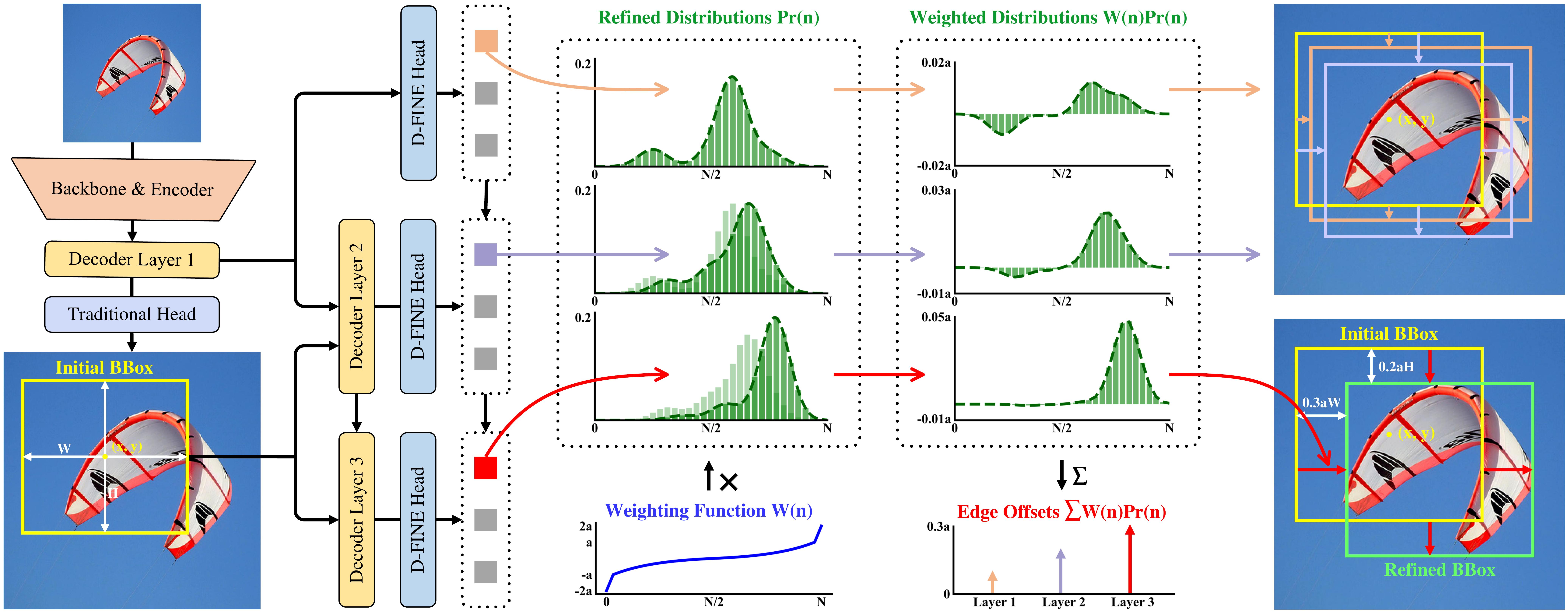
Overview of D-FINE with FDR. The probability distributions that act as a more fine- grained intermediate representation are iteratively refined by the decoder layers in a residual manner. Non-uniform weighting functions are applied to allow for finer localization.

Overview of GO-LSD process. Localization knowledge from the final layer’s refined distributions is distilled into earlier layers through DDF loss with decoupled weighting strategies.

Distributions

Visualizations of FDR across detection scenarios with initial and refined bounding boxes, along with unweighted and weighted distributions.

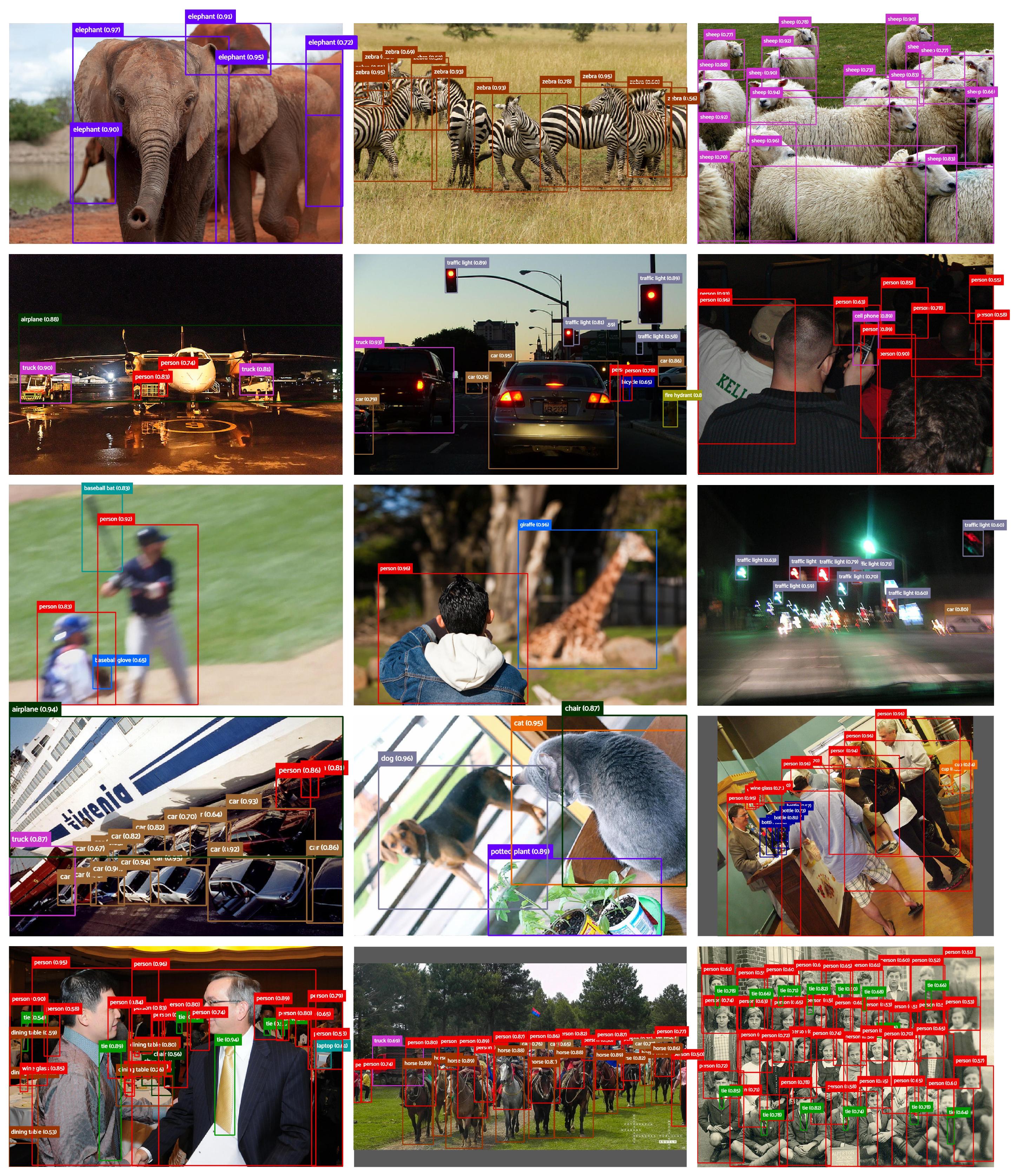
Hard Cases

The following visualization demonstrates D-FINE's predictions in various complex detection scenarios. These include cases with occlusion, low-light conditions, motion blur, depth of field effects, and densely populated scenes. Despite these challenges, D-FINE consistently produces accurate localization results.

Citation

If you use D-FINE or its methods in your work, please cite the following BibTeX entries:

bibtex

@misc{peng2024dfine,
      title={D-FINE: Redefine Regression Task in DETRs as Fine-grained Distribution Refinement},
      author={Yansong Peng and Hebei Li and Peixi Wu and Yueyi Zhang and Xiaoyan Sun and Feng Wu},
      year={2024},
      eprint={2410.13842},
      archivePrefix={arXiv},
      primaryClass={cs.CV}
}

Acknowledgement

Our work is built upon RT-DETR. Thanks to the inspirations from RT-DETR, GFocal, LD, and YOLOv9.

✨ Feel free to contribute and reach out if you have any questions! ✨

Name		Name	Last commit message	Last commit date
Latest commit History 89 Commits
.github/workflows		.github/workflows
configs		configs
reference		reference
src		src
tools		tools
.pre-commit-config.yaml		.pre-commit-config.yaml
Dockerfile		Dockerfile
LICENSE		LICENSE
README.md		README.md
README_cn.md		README_cn.md
README_ja.md		README_ja.md
requirements.txt		requirements.txt
train.py		train.py

Provide feedback

Saved searches

Use saved searches to filter your results more quickly

Repository files navigation

D-FINE: Redefine Regression Task of DETRs as Fine‑grained Distribution Refinement

🚀 Updates

Model Zoo

COCO

Objects365+COCO

Quick start

Setup

Data Preparation

Usage

Tools

Figures and Visualizations

Citation

Acknowledgement

About

Releases

Packages

Languages

License

fhandke-fugro/D-FINE

Folders and files

Latest commit

History

Repository files navigation

D-FINE: Redefine Regression Task of DETRs as Fine‑grained Distribution Refinement

🚀 Updates

Model Zoo

COCO

Objects365+COCO

Quick start

Setup

Data Preparation

Usage

Tools

Figures and Visualizations

Citation

Acknowledgement

About

Resources

License

Stars

Watchers

Forks

Releases

Packages 0

Languages

Packages