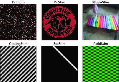
VisualStimulusToolbox 1.0.1

VisualStimulusToolbox is a lightweight MATLAB toolbox for generating, storing, and plotting 2D visual stimuli commonly used in vision and neuroscience research, such as sinusoidal gratings, plaids, random dot fields, and noise.

The toolbox allows for the easy creation, manipulation, plotting, and storing of visual stimuli such as drifting sinusoidal gratings, drifting plaids, drifting bars, random dot clouds, as well as their combinations. Every stimulus can be plotted, recorded to AVI, and stored to binary.

VisualStimulusToolbox was originally created to provide an easy way to important visual stimuli to the CARLsim spiking network simulator. As of CARLsim 3.0, it is straightforward to convert VisualStimulus .dat files to spike trains that can serve as input to CARLsim simulations. However, the toolbox can be used independently.

The toolbox is a lightweight alternative to the more comprehensive Psychophysics toolbox.

We use GitHub issues for tracking requests and bugs.

If you use this code in a scientific contribution, please consider citing it as:

Beyeler, M. "Visual Stimulus Toolbox: v1.0.0". Zenodo, June 22, 2016. doi:10.5281/zenodo.154061.

Or use the following bibtex:

@misc{visualstimulus,
  author       = {Michael Beyeler},
  title        = {Visual Stimulus Toolbox: v1.0.0},
  month        = {June},
  year         = {2016},
  doi          = {10.5281/zenodo.154061},
  url          = {http://dx.doi.org/10.5281/zenodo.154061},
  publisher    = {Zenodo}
}

Installation

You can view and manage installed add-ons in MATLAB R2016a using the Add-On Manager. To open the Add-On Manager, go to the Home tab, and select Add-Ons > Manage Add-Ons.

In older MATLAB versions, simply add the directory VisualStimulus/VisualStimulusToolbox to your MATLAB path , and you are good to go.

Getting Started

VisualStimulusToolbox provides a number of classes for creating, plotting, and storing visual stimuli such as:

• DotStim: field of randomly drifting dots
• GratingStim: drifting sinusoidal grating
• PlaidStim: drifting plaid stimulus (composed of two sinusoidal gratings)
• BarStim: drifting bar stimulus
• PictureStim: stimulus made from one or several pictures (BMP, CUR, GIF, HDF, ICO, JPEG, PBM, PCX, PGM, PNG, PPM, RAS, TIFF, XWD)
• MovieStim: stimulus made from one or several movies (AVI, MPG, MP4, M4V, MOV, WMV, MJ2, ASF, ASX)
• CompoundStim: stimulus made from a mixture of stimulus types listed above

Creating Your First Stimulus

A stimulus is intantiated by passing the desired stimulus height and width (in pixels) to the constructor:

>> dot = DotStim([120 160])
  DotStim with properties:

                  width: 160
                 height: 120
               channels: 1
                 length: 0
                   stim: []
    supportedNoiseTypes: {'gaussian'  'localvar'  'poisson'  'salt & pepper'  'speckle'}

Frames can then be added using the method add, by specifying drift direction (in degrees) and speed (in pixels/frame) as well as some other stimulus-specific options (e.g., dot density, dot coherence, dot size, etc.):

>> numFrames = 10;
>> dotSpeed = 1;
>> for dirDeg=(0:7)*45
	   dot.add(numFrames, dirDeg, dotSpeed);
   end
>> dot.plot;

This will create a stimulus made of a total of 80 frames, where dots drift into one of eight directions (in 45 degree increments) for 10 frames each.

During plotting, key events can be used to pause, stop, and step through the frames.

• Pressing p will pause plotting until another key is pressed.
• Pressing s will enter stepping mode, where the succeeding frame can be reached by pressing the right-arrow key, and the preceding frame can be reached by pressing the left-arrow key. Pressing s again will exit stepping mode.
• Pressing q will exit plotting.

Internally, the stimulus is stored as a 4D array . For example, grayscale stimuli have one channel, and RGB stimuli have three channels. The raw data array can also be accessed directly:

>> rawData4D = dot.stim;

Color stimuli can be created by passing a ColorSpec string to the constructor:

>> dot = DotStim([120 160], 'r')
                  width: 160
                 height: 120
               channels: 3
                 length: 0
                   stim: []
    supportedNoiseTypes: {'gaussian'  'localvar'  'poisson'  'salt & pepper'  'speckle'}

Currently, the following color specs are supported: 'k' (black), 'b' (blue), 'g' (green), 'c' (cyan), 'r' (red), 'm' (magenta), 'y' (yellow), and 'w' (white).

A stimulus can also be converted to an AVI movie or stored as a binary file (see below).

Manipulating an Existing Stimulus

Every stimulus type also comes with a number of handy helper methods:

• clear: Deletes all frames.
• erase: Deletes either a single frame or a list of frames.
• popFront: Deletes the first frame or number of frames.
• popBack: Deletes the last frame or number of frames.
• rgb2gray: Converts an RGB stimulus to a grayscale stimulus.
• gray2rgb: Converts a grayscale stimulus to RGB.
• resize: Resizes all frames by specifying either a scaling factor or a desired [height, width].
• addNoise: Adds noise to all existing frames. Supported noise types are given by variable supportedNoiseTypes and currently include Gaussian noise with constant mean, Gaussian white noise, Poisson noise, Salt & Pepper noise, and speckle (multiplicative) noise.

Combining Different Stimulus Types

Stimulus types can be combined to create compound stimuli. Use optional input arguments to the constructor for fast stimulus generation. For example, to combine 10 frames of drifting sinusoidal grating (120x180 pixels, red, drifting upwards and to the right at a 45 degree angle) with 20 frames of a drifting random dot cloud (240x360 pixels, blue, drifting upwards at a 90 degree angle), use the following one-liner:

>> res = GratingStim([120 180],'r',10,45) + DotStim([240 360],'b',20,90)

If the two stimuli have distinct canvas dimensions, the second stimulus will be resized to match the first stimulus' [height width]. If any of the two stimuli have more than one color channel (e.g., RGB), the result will also have more than one color channel.

Recording AVI

Every stimulus type can be converted to an AVI movie using the record method by specifying a desired file name and frame rate:

>> dot.record('myMovie.avi', 10); % 10 frames per second

Saving / Loading

Every stimulus type can be stored to a binary file, which can be loaded at a later point:

>> dot.save('myBinaryStim.dat');
>> oldStim = dot.length;
>> newDot = DotStim;
>> newDot.load('myBinaryStim.dat');
>> assert(all(oldStim(:) == newDot.stim(:)))

Acknowledgment

Some of this code is based on scripts initially authored by Timothy Saint [email protected] and Eero P. Simoncelli [email protected] at NYU for generating sinusoidal gratings, plaids, and dot clouds.

These scripts were released as part of the Motion Energy model in 2005, which was released without stating any software license restrictions. Their contributions are attributed at relevant places in the source code.