Raphael Gottardo
December 8, 2014
- It depends who you ask but, according to Wikipedia:
Bioinformatics is an interdisciplinary field that develops and improves on methods for storing, retrieving, organizing and analyzing biological data.
- Also according to Wikipedia:
Bioinformatics uses many areas of computer science, mathematics and engineering to process biological data.
-
What about statistics? Statistics plays an important role in Bioinformatics. You can't analyze data without statistics.
-
Bioinformatics is an art that involves biology, statistics, mathematics, programming, and discipline (e.g. reproducibility).
The syllabus is available on GitHub at https://github.com/raphg/Biostat-578
-
All lecture notes, R code, etc, are (will) also be available there.
-
Lecture notes are written in R markdown and processed using knitr, and thus are fully reproducible including R code and examples. The notes are fully versioned via git (and GitHub).
-
You will learn more about these tools later.
-
-
You are more than welcome to modify, correct and/or contribute. Very easy to do via pull requests. Please do not send me correction via emails.
-
Grading scheme (Tentative) HW: 40%, Midterm: 30%, Final project: 30%
Throughout this course, I will emphasize the use of open source tools for reproducible research. You might want to read the following article:
Huang, Y., & Gottardo, R. (2012). Comparability and reproducibility of biomedical data. Briefings in bioinformatics. doi:10.1093/bib/bbs078
I expect each one of you to become familiar with:
-
knitr. An R package to provide dynamic report generation with R.
-
git and GitHub. RStudio provides an integrated client for git, GitHub also provides a nice client.
We will make heavy use of these tools throughout the course.
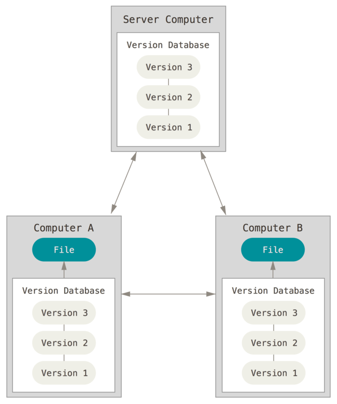
Git is version control software, it manages changes to a project without overwriting any part of that project. Great for collaborating on projects (e.g. software code).
GitHub = hosting for Git. GitHub is a social version of git, on the web with a user community. Great for finding users, collaborators, projects, but also contribute to existing project.
Some added features: Forks/Pull requests
GitHub is a great platform for bioinformatics projects. We will make extensive use of GitHub during this class, and in particular for your homework.
- Repository (repo): A repository is the most basic element of GitHub. They're easiest to imagine as a project's folder.
- Branch: A parallel version of a repository
- Clone: Local copy of the repository
- Commit: An individual change to a file (or set of files). Commits usually contain a commit message.
- Fork: A personal copy of another user's repository that lives on your account
- Merge: Merging takes the changes from one branch (in the same repository or from a fork), and applies them into another.
- Pull: Pull refers to when you are fetching in changes and merging them.
- Pull Request: Pull requests are proposed changes to a repository submitted by a user and accepted or rejected by a repository's collaborators
- Push: Pushing refers to sending your committed changes to a remote repository such as GitHub.com
- R is the son of S
- S is a statistical programming language developed by John Chambers from Bell Labs
- Goal of S was "to turn ideas into software, quickly and faithfully"
- S was created in 1976
- New S language arrived in 1988 (Blue Book) and introduced many changes (macros to functions)
- Version 4 was introduced in 1998 and introduced a formal class-method model
- In 1993, StatSci (maker of S-Plus) acquire exclusive license to S
- S-Plus integrates S with a nice GUI interface and full customer support
- R was created by Ross Ihaka and Robert Gentleman at the University of Auckland, New Zealand
- The R project started in 1991
- R first appeared in 1996 as an open-source software!
- Highly customizable via packages
- R based community, power of collaboration with thousands of packages freely available
- Many of my favorite R capabilities are not part of the base distribution
- Many graphical user interface to R both free and commercial (e.g. R studio and Revolution)
R is an integrated suite of software facilities for data manipulation, calculation and graphical display. It includes:
- an effective data handling and storage facility
- a suite of operators for calculations on arrays, in particular matrices
- a large, coherent, integrated collection of intermediate tools for data analysis
- graphical facilities for data analysis and display either on-screen or on hardcopy, and
- well-developed, simple and effective programming language which includes conditionals, loops, user-defined recursive functions and input and output facilities.
"Despite" being free and open-source, R is widely used by data analysts inside corporations and academia.
See NY Times article
<iframe src="http://www.nature.com/news/programming-tools-adventures-with-r-1.16609?WT.ec_id=NATURE-20141225"></iframe>Some references to get you started if you need to brush up your R skills.
- aRrgh: a newcomer's (angry) guide to R by Tim Smith and Kevin Ushey
- Introductory Statistics with by Peter Dalgaard
- R reference card http://cran.r-project.org/doc/contrib/Short-refcard.pdf
- R tutorial http://www.cyclismo.org/tutorial/R/
- R project and Bioconductor
More advanced:
RStudio is a free and open source integrated development environment.
- Cross platform
- Syntax highlighting, code completion, and smart indentation
- Execute R code directly from the source editor
- Easily manage multiple working directories using projects
- Plot history, zooming, and flexible image and PDF export
- Integrated with knitr
- Integrated with Git for version control
R is an overgrown calculator!
2 + 2## [1] 4
exp(-2)## [1] 0.1353353
pi## [1] 3.141593
sin(2 * pi)## [1] -2.449294e-16
You can easily find help via the command line:
help(pi)  ## equivalent ?pi
`?`(sqrt)
`?`(sin)
`?`(Special)
If you don't know the exact name, use
help.search("trigonometry")
`?`(`?`(trigonometry))
Or using the help tab integrated in RStudio, or using your favorite search engine!
Need a way to store intermediate results:
x <- 2
y <- 2
x + y
## [1] 4
Try to use meaningful names! Have a look at:
We cannot do much statistics with a single number! We need a way to store a sequence/list of numbers
One can simply concatenate elements with the c function.
weight <- c(60, 72, 75, 90, 95, 72)
weight[1]
## [1] 60
height <- c(1.75, 1.8, 1.65, 1.9, 1.74, 1.91)
bmi <- weight/height^2  ## vector based operation
bmi
## [1] 19.59184 22.22222 27.54821 24.93075 31.37799 19.73630
- Vector based operation are much faster!
ccan be used to concatenate strings and numbers.
Exercise: Find at least one other way to create a vector.
Even vectors can be limited and we need richer structures.
Homogeneous:
- Vectors (1-d)
- Matrix (2-d)
- Arrays (n-d)
Can be logical, integer, double (often called numeric), or character
Heterogeneous:
- List
- Dataframes
For more details: http://adv-r.had.co.nz/Data-structures.html
We have three types of vectors: numeric, logical, character
## Numeric vectors
x <- c(1, 5, 8)
## Logical vectors
x <- c(TRUE, TRUE, FALSE, TRUE)
## Character vectors
x <- c("Hello", "my", "name", "is", "Francis")
Exercise: Create a vector with the following elements 1, 3, 10, -1, call your vector x. Take the square root of x. Take the log of (1+x).
We have already encountered the NaN symbol meaning not-a-number, and Inf, -Inf. In practical data analysis a data point is frequently unavailable. In R, missing values are denoted by NA.
Depending on the context, R provides different ways to deal with missing values.
weight <- c(60, 72, 75, 90, NA, 72)
mean(weight)
## [1] NA
mean(weight, na.rm = TRUE)## [1] 73.8
A matrix is a two dimensional array of numbers. Matrices can be used to perform statistical operations (linear algebra). However, they can also be used to hold tables.
x <- 1:12
length(x)
## [1] 12
dim(x)## NULL
dim(x) <- c(3, 4)
x
## [,1] [,2] [,3] [,4]
## [1,] 1 4 7 10
## [2,] 2 5 8 11
## [3,] 3 6 9 12
x <- matrix(1:12, nrow = 3, byrow = TRUE)
x <- matrix(1:12, nrow = 3, byrow = FALSE)
rownames(x) <- c("A", "B", "C")
colnames(x) <- c("1", "2", "x", "y")
Matrices can also be formed by "glueing" rows and columns using cbind and rbind. This is the equivalent of c for vectors.
x1 <- 1:4
x2 <- 5:8
y1 <- c(3, 9)
my_matrix <- rbind(x1, x2)
new_matrix <- cbind(my_matrix, y1)
new_matrix
## y1
## x1 1 2 3 4 3
## x2 5 6 7 8 9
n-dimesional arrays generalize matrices, as follows:
array(1:9, c(3, 3, 3))It is common to have categorical data in statistical data analysis (e.g. Male/Female). In R such variables are referred to as factors. Makes it possible to assign meaningful names to categories. A factor has a set of levels.
pain <- c(0, 3, 2, 2, 1)
fpain <- factor(pain)
levels(fpain) <- c("none", "mild", "medium", "severe")
is.factor(fpain)
## [1] TRUE
is.vector(fpain)## [1] FALSE
## Additional attribute
levels(fpain)
## [1] "none" "mild" "medium" "severe"
A factor is very similar to an integer vector with a set of labels. While factors look like character vectors, they are not. So be careful when converting factors to characters and vice-versa. For example, use stringsAsFactors = FALSE when reading dataframes (more on this later).
Lists can be used to store objects (of possibly different kinds/sizes) into a larger composite object.
x <- c(31, 32, 40)
y <- factor(c("F", "M", "M", "F"))
## Different types and dimensions!
z <- c("London", "School")
my_list <- list(age = x, sex = y, meta = z)
my_list
## $age
## [1] 31 32 40
##
## $sex
## [1] F M M F
## Levels: F M
##
## $meta
## [1] "London" "School"
my_list$age## [1] 31 32 40
A data frame is a "data matrix" or a "data set". It is a list of vectors and/or factors of the same length that are related "across" such that data in the same position come from the same experimental unit (subject, gene, etc).
my_df <- data.frame(age = c(31, 32, 40, 50), sex = c("M", "M", "F", "M"))
my_df$age
## [1] 31 32 40 50
Why do we need data frames if it is simply a list?
- More efficient storage, and indexing!
Dataframes are similar to database tables. R provides some (more efficient) alternatives to dataframe. More later!
Name(s) of an R object can be accessed and/or modified with the names function (method).
x <- rep(1:3)
names(x)
## NULL
names(x) <- c("a", "b", "c")
my_df <- data.frame(age = c(31, 32, 40, 50), sex = y)
my_df
## age sex
## 1 31 F
## 2 32 M
## 3 40 M
## 4 50 F
names(my_df)## [1] "age" "sex"
names(my_df) <- c("age", "gender")
names(my_df)[1] <- c("Age")
Names are a special kind of attributes. See more here: http://adv-r.had.co.nz/Data-structures.html##attributes
Indexing is a great way to directly access elements of interest.
## Indexing a vector
pain <- c(0, 3, 2, 2, 1)
pain[1]
## [1] 0
pain[2]## [1] 3
pain[1:2]## [1] 0 3
pain[c(1, 3)]## [1] 0 2
pain[-5]## [1] 0 3 2 2
Note that with a data frame, the indexing of subject is straightforward!
## Indexing a matrix
my_matrix[1, 1]
## x1
## 1
my_matrix[1, ]## [1] 1 2 3 4
my_matrix[, 1]## x1 x2
## 1 5
my_matrix[, -2]## [,1] [,2] [,3]
## x1 1 3 4
## x2 5 7 8
## Indexing list is done in the same way
my_list[3]
## $meta
## [1] "London" "School"
my_list[[3]]## [1] "London" "School"
my_list[[3]][1]## [1] "London"
## Indexing a data frame
my_df[1, ]
## Age gender
## 1 31 F
my_df[2, ]## Age gender
## 2 32 M
my_list$age## [1] 31 32 40
my_list["age"]## $age
## [1] 31 32 40
my_list[["age"]]## [1] 31 32 40
my_df["Age"]## Age
## 1 31
## 2 32
## 3 40
## 4 50
## Try also my_df[1] my_df[[1]]What is the main difference between [[]] and []?
Indexing can be conditional on another variable!
pain <- c(0, 3, 2, 2, 1)
sex <- factor(c("M", "M", "F", "F", "M"))
age <- c(45, 51, 45, 32, 90)
pain[sex == "M"]
## [1] 0 3 1
pain[age > 32]## [1] 0 3 2 1
Exercise: Do the same by indexing with F. Do the same with age less than 80.
Many things in R are done using function calls, commands that look like an application of a mathematical function of one or several variables, e.g. log(x), plot(weight,height)
We will see more on this when explore advance graphics in R.
Most function arguments have sensible default and can thus be omitted, e.g. plot(weight, height, col=1)
Note: If you do not specify the names of the argument, the order is important!
R is a true programming language, and thus has a rich syntax including for loops and conditional statements (while, if, ifelse, etc).
## A simple if statement
x <- -2
if (x > 0) {
    print(x)
} else {
    print(-x)
}
## [1] 2
if (x > 0) {
    print(x)
} else if (x == 0) {
    print(0)
} else {
    print(-x)
}
## [1] 2
## For loops
n <- 1e+06
x <- rnorm(n, 10, 1)
y <- x^2
y <- rep(0, n)
for (i in 1:n) {
    y[i] <- sqrt(x[i])
}
y[1:10]
## [1] 3.218566 3.537758 3.194833 2.936778 3.226154 2.926123 3.245930
## [8] 2.913872 2.876005 3.177791
## While loops
counter <- 1
while (counter <= n) {
    y[counter] <- sqrt(x[counter])
    counter <- counter + 1
}
y[1:10]
## [1] 3.218566 3.537758 3.194833 2.936778 3.226154 2.926123 3.245930
## [8] 2.913872 2.876005 3.177791
You can easily create your own function in R. Recommended when you plan to use the same code over and over again.
## Newton-Raphson to find the square root of a number
MySqrt <- function(y) {
    x <- y/2
    while (abs(x * x - y) > 1e-10) {
        x <- (x + y/x)/2
    }
    x
}
MySqrt(81)
## [1] 9
MySqrt(101)## [1] 10.04988
For loops are notoriously slow in R, and whenever possible, it is preferable to use vectorized operations. Most functions in R are already vectorized.
## Let's generate some uniform [0,10] random numbers
n <- 10000
x <- runif(n, 0, 10)
y <- rep(0, n)
library(microbenchmark)
microbenchmark(for (i in 1:n) y[i] <- sqrt(x[i]), sqrt(x), times = 10)
## Unit: microseconds
## expr min lq mean median
## for (i in 1:n) y[i] <- sqrt(x[i]) 10160.222 10396.59 12069.0914 10919.690
## sqrt(x) 44.473 47.65 54.7425 48.083
## uq max neval cld
## 13569.264 18215.223 10 b
## 55.094 80.908 10 a
The for loop is increadibly slower!
While you will often hear that R is slow, there are many ways to speed up calculations in R, often by using third party libraries (e.g. data.table, Rcpp).
The *apply family of functions is intended to try to solve some of the side effects of for loops, such as facilitating it's application to R objects (e.g. lists) and improving efficiency.
The most common *apply functions are
-
apply: Returns a vector or array or list of values obtained by applying a function to margins of an array or matrix. -
lapply: apply a function or each element of a list or vector -
sapply: a user-friendly version and wrapper of lapply by default returning a vector, matrix or, an array. sapply will try to guess what the output should be based on the input.
For more details have a look at this.
## Let's generate some uniform [0,10] random numbers
n <- 10000
x <- runif(n, 0, 10)
y <- rep(0, n)
library(microbenchmark)
microbenchmark(for (i in 1:n) y[i] <- MySqrt(x[i]), sapply(x, MySqrt), times = 10)
## Unit: milliseconds
## expr min lq mean median
## for (i in 1:n) y[i] <- MySqrt(x[i]) 58.08852 60.16150 64.20910 61.40455
## sapply(x, MySqrt) 51.92839 53.71897 62.29996 57.55061
## uq max neval cld
## 63.04317 88.50716 10 a
## 71.19711 89.74499 10 a
*apply functions are not necessarily faster than for loops, but they can be very convenient and usually lead to more compact and more elegant code.
More efficiency gain can be obtained using compiled code (e.g. C++). R provides multiple ways to call compiled code. In particular, the Rcpp package can greatly facilitate the use of C++ compiled code.
Exercise: Write some code to use the apply function on a given matrix.
- Approach to programming introduced by Donald Knuth
- An explanation of a program logic in a plain English, interspersed with chunk of computer code.
- Sweave
- Create dynamic reports by embedding R code in latex documents
- Sweave is good but ...
- Writing latex is painful
- Output is limited to pdf
- knitr
- Transparent engine for dynamic report generation
- knitr allows any input languages (e.g. R, Python and Awk) and any output markup languages
- Full control of input, code, and output
- Fine control over how the code is executed and the ouput is displayed
- knitr can process input files in various formats: latex, html, R markdown
- R markdown
- markdown: easy-to-read, easy-to-write plain text format that can be converted to html
- R markdown: markdown + R code chunks
- R presentation
- knitr is readily accessible in RStudio
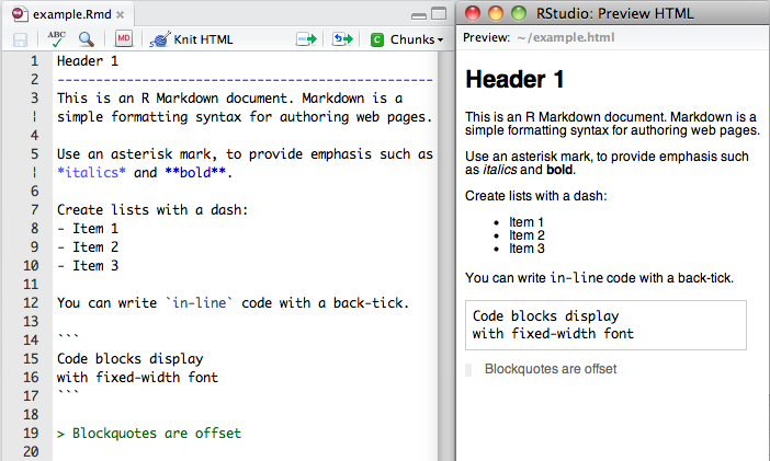
Markdown is a simple markup language similar to wiki markups
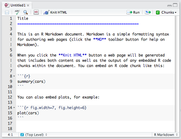
Mardown with R code chuncks.
As we've seen, R expressions can also be evaluated inline:
pi=3.1415927
Large data and complex analysis can require significant computing time
- Not unusual for an analysis to take a few minutes to an hour, or even more!
- This can result in some performance issues when viewing a report → User frustration
- Why rerun a script when nothing has changed?
- The solution is caching
knitr provides powerful caching mechanism:
- cache can be turned on/off for each code chunk
- If caching is on, knitr will check if the code has changed when rerunning a report
- Chunks can be made dependent
- The caching mechanism is flexible can be attached to an R version, an input dataset, a date, etc.
What you need to do:
- Download R and RStudio
- Signup for an account on GitHub.
- Set up your first repository!
- Try knitr and git within RStudio
We will use RStudio, GitHub and knitr a whole lot throughout this course!
I expect your to use GitHub/knitr/Rstudio for your homeworks and final project!


