project2_ekf_slam

Project 2 - EKF SLAM

Introduction

In Project 2, you’ll be required to implement the extended Kalman filter for a 2D landmark-based SLAM system. You’ll receive a ROS package, ekf_slam, which contains skeleton code for the filter. You’ll need to follow the instructions detailed in the last page, step by step

Instruction

In the prediction phase, we provide two key parameters: the velocity of axis $X$ and the angular velocity of axis $Z$. These are stored in the variable $ut$ of the EKFSLAM::run function. Given the differential wheeled robot model, only these two values should be non-zero in theory. We also assume that there are noises in both values, represented by $σv$ and $σω$. The interval time is denoted by $dt$.

In the update phase, you’ll be given code for cylinder detection. This code generates a set of 2D coordinates for the centers of detected cylinders in the body frame. These are represented by Eigen::MatrixX2d cylinderPoints. Your task is to associate cylinder observations with your landmarks in the state and to use observed cylinders to update your pose and landmarks. If a new observation occurs, you should augment your state and covariance matrix. Remember to keep the angle between $-pi$ and $pi$

Every section of the package that requires your implementation is marked by TODO. If you’re unsure of your next steps, searching for TODO globally in the package could help guide you. If you encounter a bug, a useful debugging strategy is to print out as much information as possible.

ekf_slam

cd /ws
catkin_make
source devel/setup.bash
roslaunch ekf_slam ekf_slam.launch
# Press `blankspace` to start the odometry estimation

Evaluation

You can evaluate the performance of your implementation by comparing the estimated odometry with the ground truth. Recommended to use evo to evaluate the performance.

1. Record the rosbag data with estimated odometry and ground truth odometry.

rosbag record /slam_node/ekf_odom /odom -O ekf_odom.bag

2. Run evo to evaluate the performance.

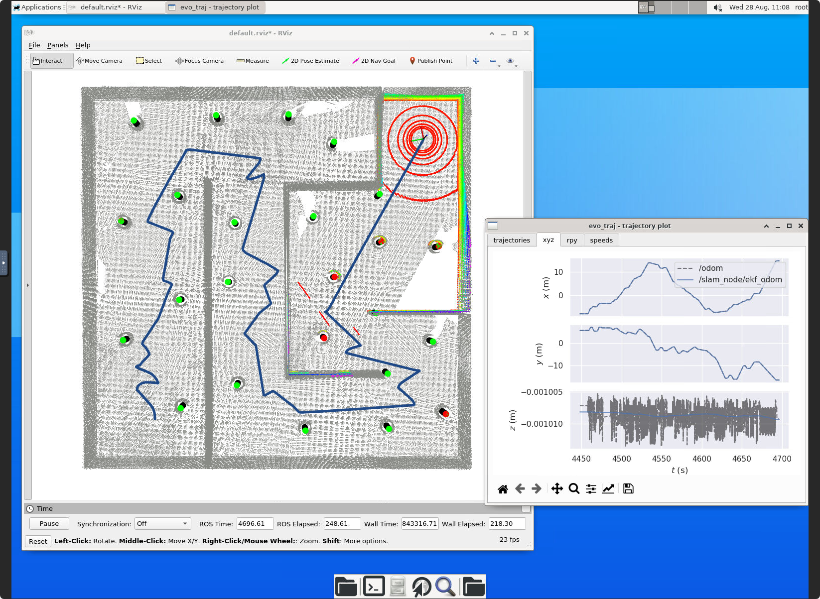
evo_traj bag ekf_odom.bag /slam_node/ekf_odom --ref /odom -a -p
evo_ape bag ekf_odom.bag xxxxxxxxx
evo_rpe bag ekf_odom.bag xxxxxxxxx

example of evo_traj:

Scoring Rules

1. Please title your submission "PROJECT2-YOUR-NAMES.zip". Your submission should include a maximum 2-page report and all necessary files to run your code, a video in 1 minute, rosbag with the estimated odometry and ground truth odometry.
2. The report should contain at least a visualization of your final point cloud map and trajectory.
3. If your code is similar to others’ or any open-source code on the internet, the score will be 0 unless the sources are properly referenced in your report. Refer to $^1$ for details.
4. Excessive white space, overly large images, or redundant descriptions in report will not contribute to a higher score. Simple but efficient code is preferred.
5. If any problem, please google first. If unsolved, create a discussion on Canvas.
6. If you have no experience of C++ coding, start this project as early as possible. Programming proficiency is not determined by the courses you’ve taken, but rather by ample practice and persistent debugging.
7. Submit your code and documents on Canvas before the deadline. Scores will be deducted for late submission.

References

[1] https://registry.hkust.edu.hk/resource-library/academic-integrity

Appendix

Prediction

State:

$$\mu=\left[\begin{array}{llllll}x & y & \theta & m_{1} & \ldots & m_{n}\end{array}\right]^{T} \quad \Sigma=\left[\begin{array}{ll}\Sigma_{x x} & \Sigma_{x m} \\ \Sigma_{m x} & \Sigma_{m m}\end{array}\right]$$

Robot control:

$$u_{t}=\left[\begin{array}{l}v_{x} \\ \omega_{z}\end{array}\right], n=\left[\begin{array}{l}\sigma_{v} \\ \sigma_{\omega}\end{array}\right], R_{n}=cov(n)$$

Motion function:

$$\bar{\mu}_{t}=\mu_{t-1}+B u_{t}$$ $$\bar{\Sigma}_{t}=G_{t} \Sigma_{t-1} G_{t}^{T}+F_{t} R_{n} F_{t}^{T}$$ $$B=F_{t}=\left[\begin{array}{cc}\Delta t \cos \left(\theta_{t-1}\right) & 0 \\ \Delta t \sin \left(\theta_{t-1}\right) & 0 \\ 0 & \Delta t \\ 0 & 0 \\ \vdots & \vdots \\ 0 & 0\end{array}\right] G_{t}=\left[\begin{array}{cccccc}1 & 0 & -v_{x} \Delta t \sin \left(\theta_{t-1}\right) & 0 & \cdots & 0 \\ 0 & 1 & v_{x} \Delta t \cos \left(\theta_{t-1}\right) & \vdots & \ddots & \vdots \\ 0 & 0 & 1 & 0 & \cdots & 0 \\ 0 & \cdots & 0 & 1 & \cdots & 0 \\ \vdots & \ddots & \vdots & \vdots & \ddots & \vdots \\ 0 & \cdots & 0 & 0 & \cdots & 1\end{array}\right]$$

Update

$$\begin{equation} H_t=\frac{1}{q}\left[\begin{array}{ccccc} -\sqrt{q} \delta_x & -\sqrt{q} \delta_y & 0 & \sqrt{q} \delta_x & \sqrt{q} \delta_y \\\ \delta_y & -\delta_x & -q & -\delta_y & \delta_x \end{array}\right]\left[\begin{array}{ccccccc} 1 & 0 & 0 & 0 & 0 & 0 & 0 \\\ 0 & 1 & 0 & 0 & 0 & 0 & 0 \\\ 0 & 0 & 1 & 0 & 0 & 0 & 0 \\\ 0 & 0 & 0 & 0 & 1 & 0 & 0 \\\ 0 & 0 & 0 & \underbrace{0}_{2 \cdot j-2} & 0 & 1 & \underbrace{0}_{2 n-2 j} \end{array}\right] \quad \begin{aligned} & K_t=\bar{\Sigma}_t H_t^T\left(H_t \bar{\Sigma}_t H_t^T+Q\right)^{-1} \\\ & \mu_t=\bar{\mu}_t+K_t\left(z_t-\hat{z}_t\right) \\\ & \Sigma_t=\left(I-K_t H_t\right) \bar{\Sigma}_t \end{aligned} \end{equation}$$