- Abstract
- What is Transfer Learning?
- Use Cases of Transfer Learning
- Popular Pre-Trained Models for Transfer Learning
- Comparative Case-Study of VGG16, ResNet and Inception v3 models
- Conclusion
Binary classification is one of the most common and frequently tackled problems in the deep learning domain. It is generally applied when the user wants to classify an entity into one of the two possible categories. The difference between binary & multi-class classification is aptly showed in following snippet:
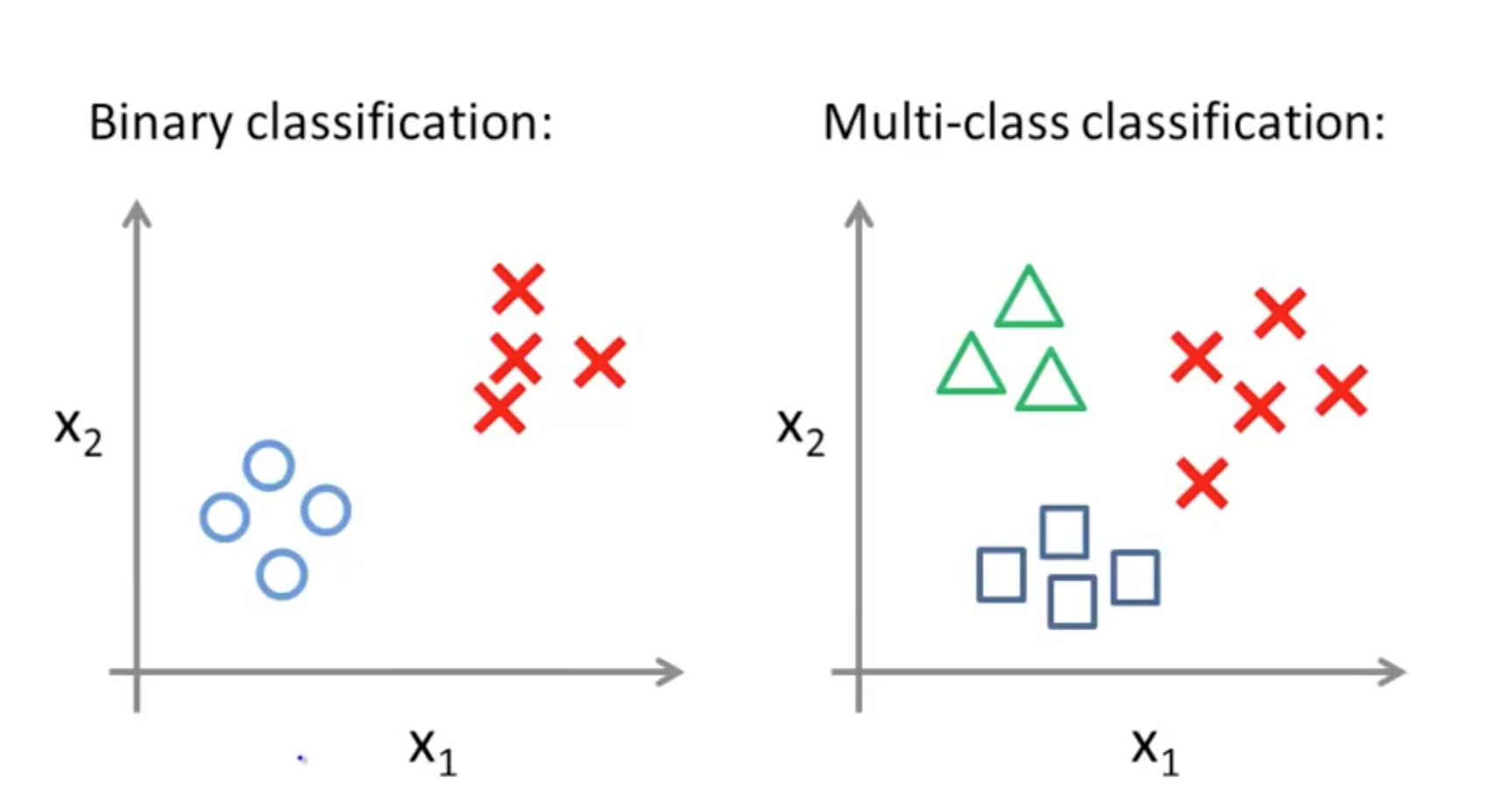
As shown in the above snippet, when we are provided dataset of labelled images into two categories(or two different clusters per se), binary classification is applied. Though this seems like a trivial task, it does involve fair amount of underlying computation. This computation is based on incorporating the principles used for efficient classification by ‘Intelligent Algorithms.’ One of those intelligent algorithms are Neural Networks. Through the effective use of neural networks, binary classification problems can be solved to a fairly high degree. In this literature survey, we are going to observe how Transfer Learning improves the performance of a neural network based deep learning model.
Transfer Learning is the reuse of a pre-trained model on a new but similar problem. Basically, in transfer learning, a machine exploits the knowledge gained from a previous task to improve generalization about another i.e we transfer the weights that a network has learned in the previous task to the new task.
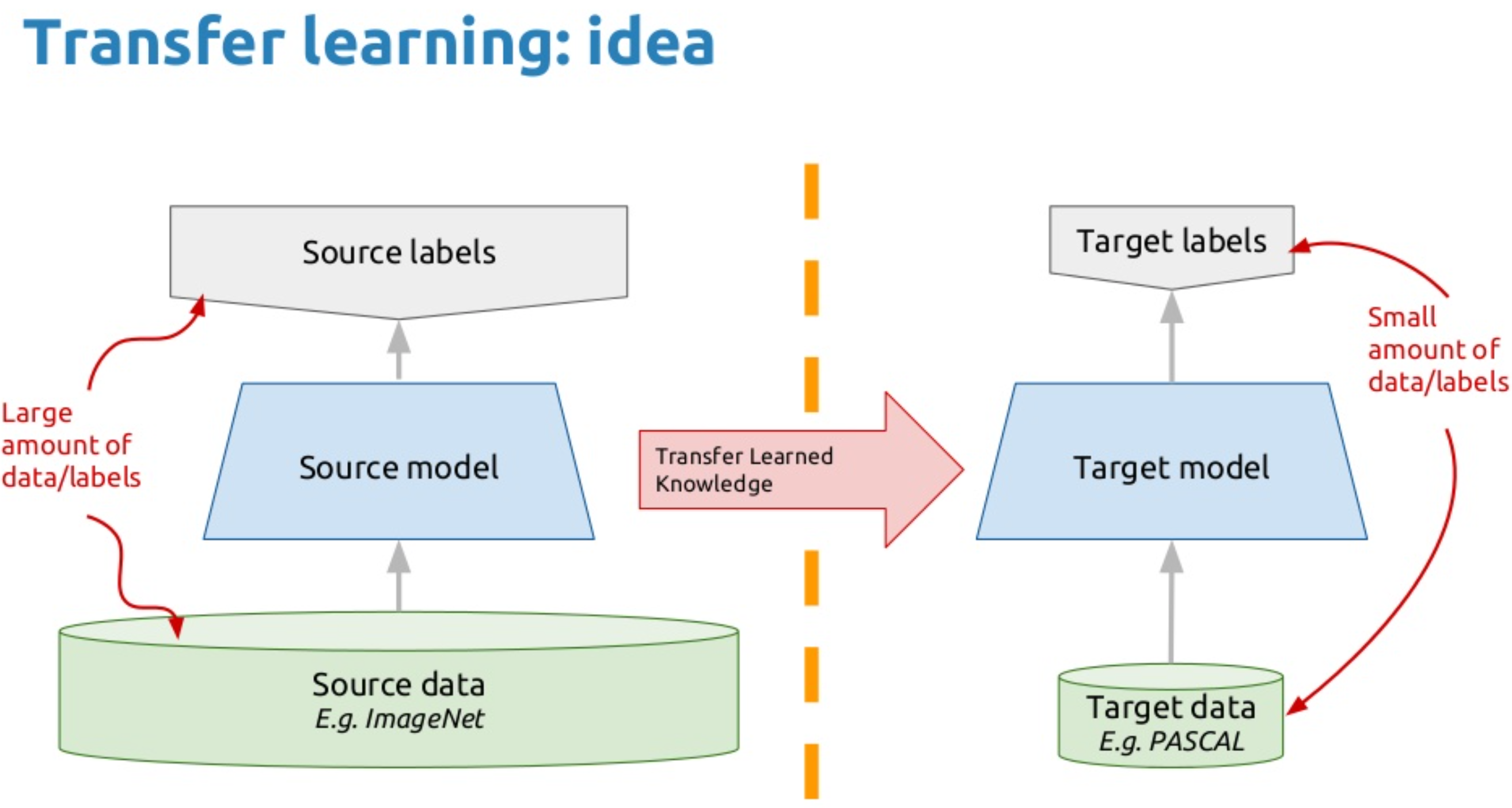
It's currently very popular in deep learning because it can train deep neural networks with comparatively little data. This is very useful in the data science field since most real-world problems typically do not have millions of labelled data points to train such complex models.
The general use case for using transfer learning is when we need to use the knowledge a model has learned from a task with a lot of available labelled training data in a new task that doesn't have much data. So that instead of starting the learning process from scratch, we start with patterns learned from solving a related task.
Transfer learning is mostly used in computer vision and natural language processing tasks like sentiment analysis due to the huge amount of computational power required. Transfer learning has several benefits, but the main advantages are saving training time, better performance of neural networks (in most cases), and not needing a lot of data.
Some of the very popular pre-trained models for Transfer Learning are as follows:
- VGG-16
- ResNet
- Inception v3
VGG16 is a convolutional neural network model proposed by K. Simonyan and A. Zisserman from the University of Oxford in the paper “Very Deep Convolutional Networks for Large-Scale Image Recognition”. The model achieves 92.7% top-5 test accuracy in ImageNet, which is a dataset of over 14 million images belonging to 1000 classes. It was one of the famous model submitted to ILSVRC-2014. As a result, the network has learned rich feature representations for a wide range of images. It makes the improvement over AlexNet by replacing large kernel-sized filters (11 and 5 in the first and second convolutional layer, respectively) with multiple 3×3 kernel-sized filters one after another. VGG16 was trained for weeks and was using NVIDIA Titan Black GPU’s.

The input to conv1 layer is of fixed size 224 x 224 RGB image. The image is passed through a stack of convolutional (conv.) layers, where the filters were used with a very small receptive field: 3×3 (which is the smallest size to capture the notion of left/right, up/down, center). In one of the configurations, it also utilizes 1×1 convolution filters, which can be seen as a linear transformation of the input channels (followed by non-linearity). The convolution stride is fixed to 1 pixel; the spatial padding of conv. layer input is such that the spatial resolution is preserved after convolution, i.e. the padding is 1-pixel for 3×3 conv. layers. Spatial pooling is carried out by five max-pooling layers, which follow some of the conv. layers (not all the conv. layers are followed by max-pooling). Max-pooling is performed over a 2×2 pixel window, with stride 2.
Three Fully-Connected (FC) layers follow a stack of convolutional layers (which has a different depth in different architectures): the first two have 4096 channels each, the third performs 1000-way ILSVRC classification and thus contains 1000 channels (one for each class). The final layer is the soft-max layer. The configuration of the fully connected layers is the same in all networks.
All hidden layers are equipped with the rectification (ReLU) non-linearity. It is also noted that none of the networks (except for one) contain Local Response Normalisation (LRN), such normalization does not improve the performance on the ILSVRC dataset, but leads to increased memory consumption and computation time.
ResNet is a short name for Residual Network. ResNet makes it possible to train up to hundreds or even thousands of layers and still achieves compelling performance. Taking advantage of its powerful representational ability, the performance of many computer vision applications other than image classification have been boosted, such as object detection and face recognition.
The ResNet network can take the input image having height, width as multiples of 32 and 3 as channel width. For the sake of explanation, we will consider the input size as 224 x 224 x 3. Every ResNet architecture performs the initial convolution and max-pooling using 7×7 and 3×3 kernel sizes respectively. Afterward, Stage 1 of the network starts and it has 3 Residual blocks containing 3 layers each. The size of kernels used to perform the convolution operation in all 3 layers of the block of stage 1 are 64, 64 and 128 respectively. The curved arrows refer to the identity connection. The dashed connected arrow represents that the convolution operation in the Residual Block is performed with stride 2, hence, the size of input will be reduced to half in terms of height and width but the channel width will be doubled. As we progress from one stage to another, the channel width is doubled and the size of the input is reduced to half. The workflow of ResNet is as below:

For deeper networks like ResNet50, ResNet152, etc, bottleneck design is used. For each residual function F, 3 layers are stacked one over the other. The three layers are 1×1, 3×3, 1×1 convolutions. The 1×1 convolution layers are responsible for reducing and then restoring the dimensions. The 3×3 layer is left as a bottleneck with smaller input/output dimensions.
Finally, the network has an Average Pooling layer followed by a fully connected layer having 1000 neurons (ImageNet class output).
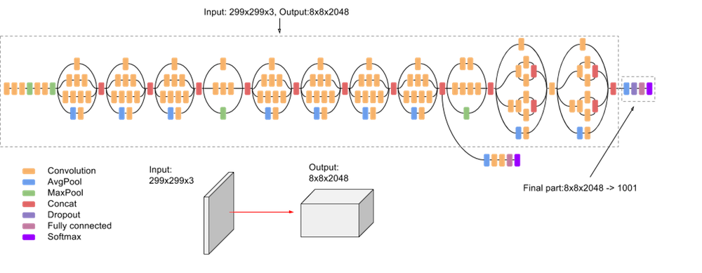
Inception V3 by Google is the 3rd version in a series of Deep Learning Convolutional Architectures. Inception V3 was trained using a dataset of 1,000 classes (See the list of classes here) from the original ImageNet dataset which was trained with over 1 million training images, the Tensorflow version has 1,001 classes which is due to an additional "background' class not used in the original ImageNet. Inception V3 was trained for the ImageNet Large Visual Recognition Challenge where it was a first runner up. The paper proposes a new type of architecture – GoogLeNet or Inception v1. It is basically a convolutional neural network (CNN) which is 27 layers deep.
Notice in the above image that there is a layer called inception layer. This is actually the main idea behind the approach. The inception layer is the core concept of a sparsely connected architecture.
Inception Layer is a combination of all those layers (namely, 1×1 Convolutional layer, 3×3 Convolutional layer, 5×5 Convolutional layer) with their output filter banks concatenated into a single output vector forming the input of the next stage.
Wherein the inception layer looks like this:
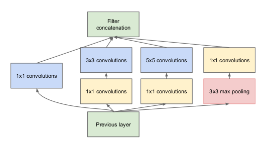
Along with the above-mentioned layers, there are two major add-ons in the original inception layer:
- 1×1 Convolutional layer before applying another layer, which is mainly used for dimensionality reduction
- parallel Max Pooling layer, which provides another option to the inception layer.
The weights for Inception V3 are smaller than both VGG and ResNet, coming in at 96MB.
- Inception is created to serve the purpose of reducing the computational burden of deep neural nets while obtaining state-of-art performance. As the network goes deeper, the computational efficiency will also decrease, therefore the authors of Inception were interested in finding a solution to scale up neural nets without increasing computational cost.
- While Inception focuses on computational cost, ResNet focuses on computational accuracy. Intuitively, deeper networks should not perform worse than the shallower networks, but in practice, the deeper networks performed worse than the shallower networks, caused not by overfitting, but by an optimization problem.
- Shortly, the deeper the network, the harder the network to be optimized.
This table compares the performace of all the three models and their upgradation in the classic ILSVRC as follows:

✔️ The trend in the computer vision is to make deeper and more complicated network to achieve higher accuracy. However, deeper networks come with the tradeoff of size and speed. In real applications such as an autonomous vehicle or robotic visions, the object detection task must be able to be done on the computationally limited platform.